Calibration Science, Part II: Systematic Error, Signal-to-Noise Ratios, and How to Reduce Random Error

In this, the second installment of the calibration science series, we will introduce a second type of error besides random error, called systematic error. We will see how accuracy measures both types of error, discuss how to quantitate error by measuring signal-to-noise ratios, and how to improve data quality despite the presence of error by averaging observations together.

From Last Time

In the first installment of this series, (1) we covered precision and accuracy and the fact that that they are different. We also covered some of this ground early on in the history of the cannabis analysis columns (2) but will go into more detail here. The concepts of precision and accuracy are illustrated in Figure 1.

The bullseye in Figure 1 represents the true value of the quantity being measured, and the seven data points are repeat measurements of the same quantity.

Precision is a measure of the spread in a series of measurements of the same quantity. Accuracy is a measure of how far you are off from the true value. The leftmost target in Figure 1 shows data that are imprecise because it is scattered all over the place. This scatter in the data is called by many names including dispersion and variance. These data are inaccurate because the data points are on average far away from the true value. The middle target in Figure 1 shows data that is precise but inaccurate. The data are precise because the seven measurements are all clustered close together. However, the data are inaccurate because they are centered far from the bullseye. This target is key to understanding that precision and accuracy are different things. The rightmost target in Figure 1 shows data that is precise and accurate because the data are tightly clustered together and are centered on the bullseye.

Another concept introduced previously is that of random error. Random error is caused by variables in the universe that we do not always have control over, a list of which was given last time (1).

Systematic Error

The second type of error that can be present in data is systematic error. Systematic error means that a measurement is always off by the same amount in the same direction from the true value. Systematic error is also known as bias. A classic example of systematic error is when you forget to reset your clock when Daylight Savings time happens in the Spring (remember “spring ahead, fall back”). If you forget to reset your clock it will always be an hour behind the rest of the country, always off by the same amount, and it will always be off in the same direction, always an hour slow. The beauty of systematic error is that it is easy to spot and correct. In the case of our clock, the systematic error can be eliminated by simply setting the clock forward an hour. In other types of data, if you know there is bias, for example, all the potency measurements from your chromatograph are high by 1% tetrahydrocannabinol (THC), the solution is simply to subtract 1% from all the THC measurements made with this instrument.

Quoting Error

The sign of random noise is random, that is, its sign varies between being positive and negative randomly over time. Therefore, we quote the error in a measurement as ± whatever the error is. For example, the magnitude and error in the chromatographic determination of the THC level in a cannabis bud may be 20 ±0.1 wt. %. The ±0.1 is also called the margin of error, a term you might have heard in reference to opinion polls. The margin of error is often times quoted as half the total error because the spread in measured values can equally likely be above or below the true value. All measurements and margins of error should be quoted with the correct number of significant figures, a topic we have covered previously (3).

Signal-to-Noise Ratio (SNR)

Another measure of data quality other than precision and accuracy is the
signal-to-noise ratio or SNR for short. The SNR is the ratio of the magnitude of the thing being measured to the error in the measurement as seen in Equation 1:

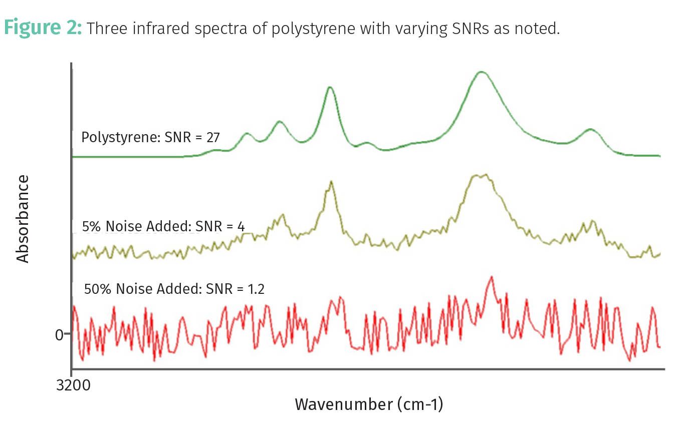
The signal in this case could be, for example, the peak height or area of a chromatographic or spectroscopic peak. This is illustrated by the infrared spectra of a polystyrene sample seen in Figure 2.

The top spectrum in green has an SNR of 27. Note that the peaks are easy to see here. The middle spectrum in brown has an SNR of 4. The random, jagged up and down stuff you see is noise; pretty ugly, isn’t it? In this case, the polystyrene peaks are discernible but just barely above the noise level. The bottom spectrum in red has an SNR of 1.2. In this situation, the peaks and the noise are about the same magnitude, and it is next to impossible to see the polystyrene peaks.

In general, a peak in a spectrum or chromatogram is considered real if it has an SNR of >= 3, but this is the bare minimum. Spectrometers and chromatographs are capable of SNRs of 100 or greater, and data of this high quality should always be your goal. SNR values can also be used in the calculation of limits of quantitation and detection, which we will discuss in a future column.

How to Reduce Random Noise

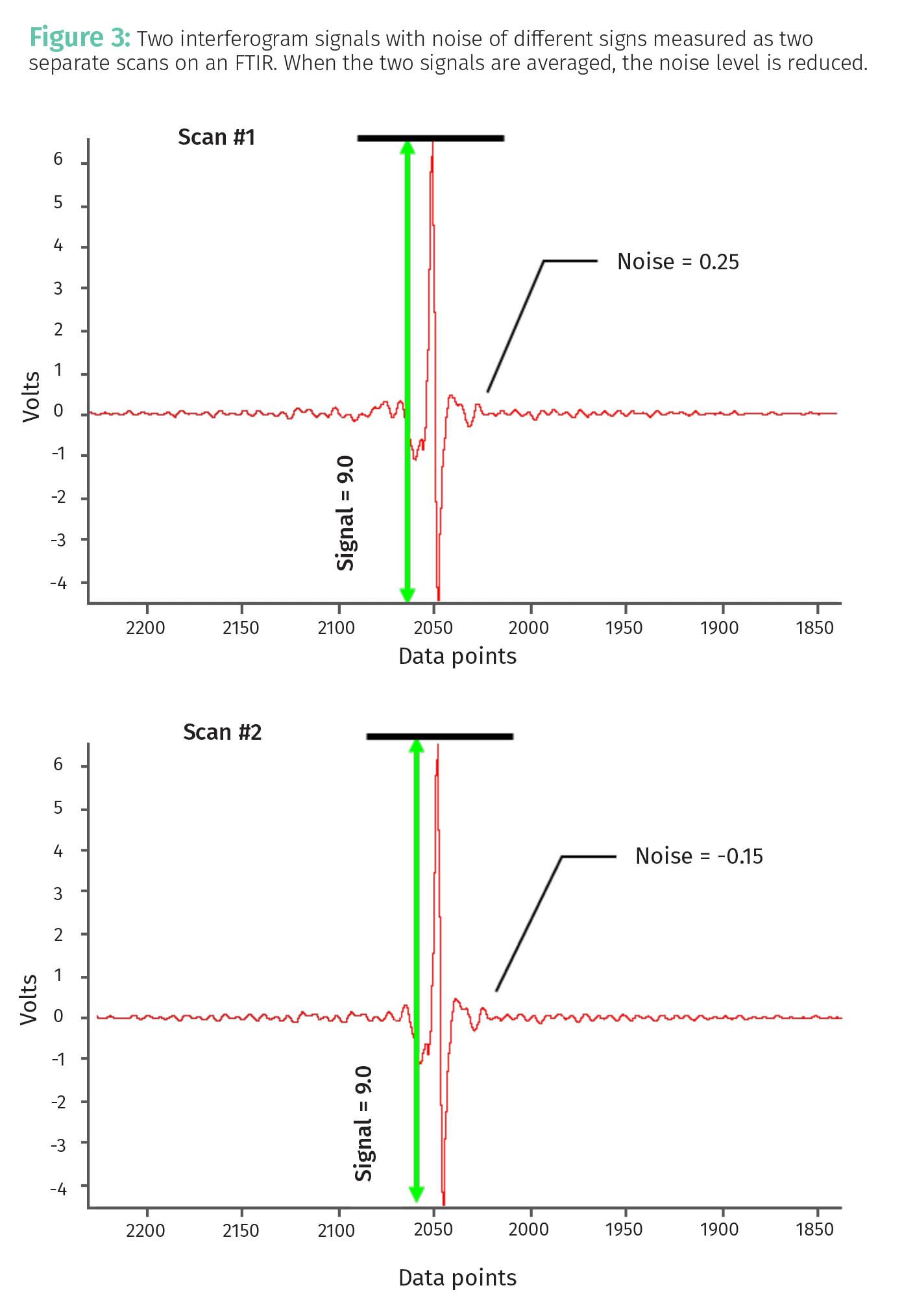
Now that we have discussed the many sources of random noise, the real question is how to reduce it. Of course, use of well-calibrated instruments and careful experimentation are one way to reduce noise. However, there will always be noise in your measurements. What do we do then? We take advantage of the fact that the sign of random noise is random as illustrated in Figure 3.

Seen are two raw signals from the detector on an infrared spectrometer. These are called interferograms, and these two scans were measured on a Fourier transform infrared spectrometer (FTIR) (4) one right after the other. These signals could just easily be from the detector on a chromatograph—the principles here are all the same. Note that in the two interferograms the signal is the same, a value of 9 V, which means the instrument and sample are stable, always a good thing. However, note that in the first scan the noise level is 0.25 and in the second scan it is -0.15. When we average the two scans, we obtain the result seen in
Equation 2:

Note that the average noise, 0.05, is less than the absolute value of either of the individual noise measurements, namely 0.25 and 0.15. Averaging observations works because when the positive and negative going noise points are added together, they have a tendency to cancel each other.

The key then to reducing random noise is to average multiple observations together. In FTIR this is done by averaging scans; for measuring potency or pesticide levels in cannabis samples this means analyzing multiple aliquots of the same sample and averaging them together. As it turns out, SNR and the number of observations averaged together are proportional to each other as given by Equation 3:

where SNR is the Signal-to-Noise Ratio and N is the number of observations averaged together.

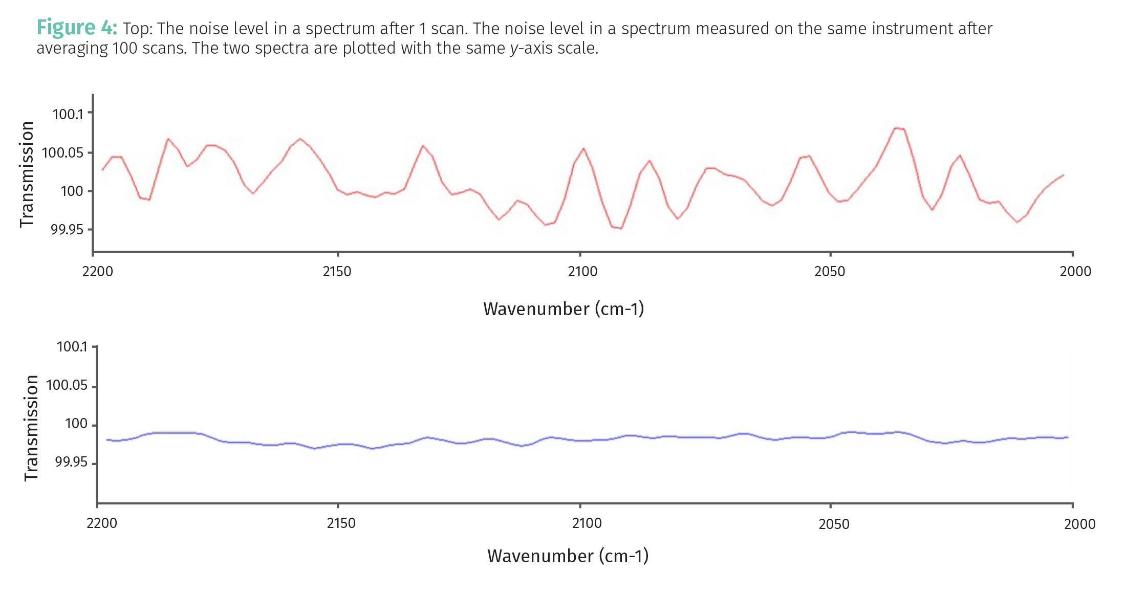
Note then that SNR improves with the square root of the number of observations averaged together. This is illustrated in Figure 4.

The top spectrum in Figure 4 shows the noise in a spectrum measured with an FTIR using one scan. The random, jagged, up and down ugliness that is noise, is clearly seen. The bottom spectrum in Figure 4 shows the noise level measured on the same instrument under the same conditions except that 100 scans were averaged together. The two spectra in Figure 4 were plotted using the same y-axis limits and so can be compared to each other. Note that the amount of noise is significantly reduced in the bottom spectrum. Using Equation 3, we would expect the bottom spectrum to have (100)^1/2 or 10 times less noise than the top spectrum. I confirmed this by measuring the noise levels in the two spectra. Yes, averaging measurements really reduces random noise.

I realize that for things like pesticide and potency measurements on cannabis samples, obtaining 100 analyses of the same sample and averaging is nigh impossible. However, even averaging 3 measurements helps. For example, let’s say the THC level in a cannabis bud is measured as 20±2%. If we averaged 3 measurements of the THC levels in this sample, we would expect the noise level to be reduced by (3)^1/2 or a factor of 1.73. The margin of error then for the average THC value would be (2/1.73) = 1.2, which we would write as 20±1.2%. We have almost halved the error in the THC measurement by simply analyzing 3 aliquots instead of one. I strongly recommend that cannabis labs run their samples in duplicate or triplicate and average the results to reduce the amount of error in their measurements.

Conclusions

Systematic error, or bias, is when a measurement is always off from the true value by the same amount in the same direction. Unlike random error which cannot be completely corrected, systematic error can be eliminated by adding or subtracting the known bias from each measurement.

The SNR is a measure of data quality and is simply the size of a measurement divided by the noise in that measurement. Naturally, SNR is something we want to maximize. This can be done by averaging observations together to reduce the random noise. We saw that the SNR improvement goes as the square root of the number of measurements added together.

References

1. Smith, B., Calibration Science, Part I: Precision, Accuracy, and Random Error, Cannabis Science and Technology, 2023, 6(9), 6-9.
2. Smith, B., Error, Accuracy, and Precision, Cannabis Science and Technology, 2018, 1(4), 12-16.
3. Smith, B., Significant Figures and Margin of Error-Or Why the Fourth Decimal Place in Your Potency Reading is Probably Meaningless, Cannabis Science and Technology, 2020, 3(4), 10–12.
4. Smith, B., Fundamentals of Fourier Transform Infrared Spectroscopy, CRC Press, 2011.

About the Columnist

Brian C. Smith, PhD, is Founder, CEO, and Chief Technical Officer of Big Sur Scientific. He is the inventor of the BSS series of patented mid-infrared based cannabis analyzers. Dr. Smith has done pioneering research and published numerous peer-reviewed papers on the application of mid-infrared spectroscopy to cannabis analysis, and sits on the editorial board of Cannabis Science and Technology. He has worked as a laboratory director for a cannabis extractor, as an analytical chemist for Waters Associates and PerkinElmer, and as an analytical instrument salesperson. He has more than 30 years of experience in chemical analysis and has written three books on the subject. Dr. Smith earned his PhD on physical chemistry from Dartmouth College.
Direct correspondence to: brian@bigsurscientific.com.

How to Cite this Article

Smith, B., Calibration Science, Part II: Systematic Error, Signal-to-Noise Ratios, and How to Reduce Random Error, Cannabis Science and Technology, 2024, 7(1), 8-11.