Error, Accuracy, and Precision

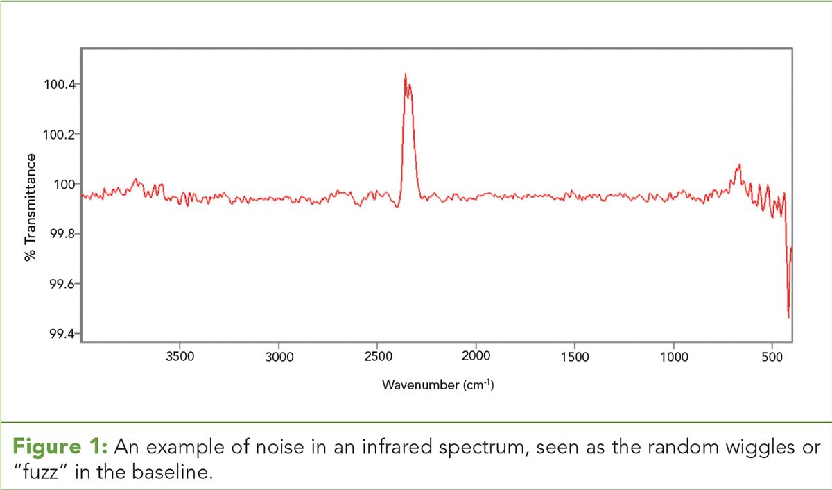
Figure 1: An example of noise in an infrared spectrum, seen as the random wiggles or “fuzz” in the baseline.

In the science of analytical chemistry, we quantitate things such as weights and concentrations. All of these measurements generate a number, but to truly understand the quality of data we have to know the size of the error in the measurement. Well known measures of data quality include accuracy and precision. Do you know the difference between these two metrics? Do you know how to quantitate them? And how does all of this apply to cannabis analysis? Please read on to find out more.

Any time a quantity is measured, be it your weight on a bathroom scale, the speed of light, or potency of a cannabis bud, there will be error involved in the measurement. Sources of error include environmental changes, power fluctuations, electronics, and good old fashioned human error. Error exists because human beings are not gods and thus cannot control all the variables all the time for any given measurement (1). Two of the most important types of noise are random noise and systematic noise. Let’s discuss random noise first.

Random Noise

Random error is caused by variables we cannot control as mentioned above. The sign of random error is random, that is, it is equally probable to be positive or negative. This is why measurements are often times expressed as X±y, where X represents the value of the measurement and y represents the amount of error in the measurement. Error is sometimes called noise, and the quality of data can be expressed as a signal-to-noise ratio (SNR) defined in equation 1.

SNR = (Signal)/(Noise)               [1]

The SNR concept is perhaps best illustrated using a cell phone call. In this case, the volume of the caller’s voice is the signal and the static in the connection is the noise. If the volume of the caller’s voice is large compared to the static, the connection has a good SNR and you can clearly hear what the other person is saying. Alternatively, if the static in the connection is high, and the caller’s voice can barely be heard above it, the SNR of the call is low and you will have trouble understanding what your caller is saying. Note that a high SNR phone call, or any high SNR data, will carry a lot of information. Whereas a low SNR phone call or low SNR data will carry very little information. This is why SNR is a measure of data quality.

In analytical chemistry error is often seen as “fuzz” in the baseline of chromatographic and spectroscopic measurements. An example of this is seen in Figure 1. (See upper right for Figure 1, click to enlarge. Figure 1: An example of noise in an infrared spectrum, seen as the random wiggles or “fuzz” in the baseline.)

Figure 1 shows noise measured by a Fourier transform-infrared (FT-IR) spectrometer. Since the sign of random noise is random, the baseline fluctuates up and down randomly. The size of these wiggles is a measure of the noise (2). Note in Figure 1 that the size of the noise varies with wavenumber, which is typical of any spectrum measured using light (electromagnetic radiation).

The big peak at 2350 cm^-1 in Figure 1 is an artifact, which is a peak or signal in your data that is not from the sample. This peak is from the presence of unwanted atmospheric carbon dioxide inside the instrument. If you see a CO₂ peak in an FT-IR spectrum that you measure, it is an artifact.

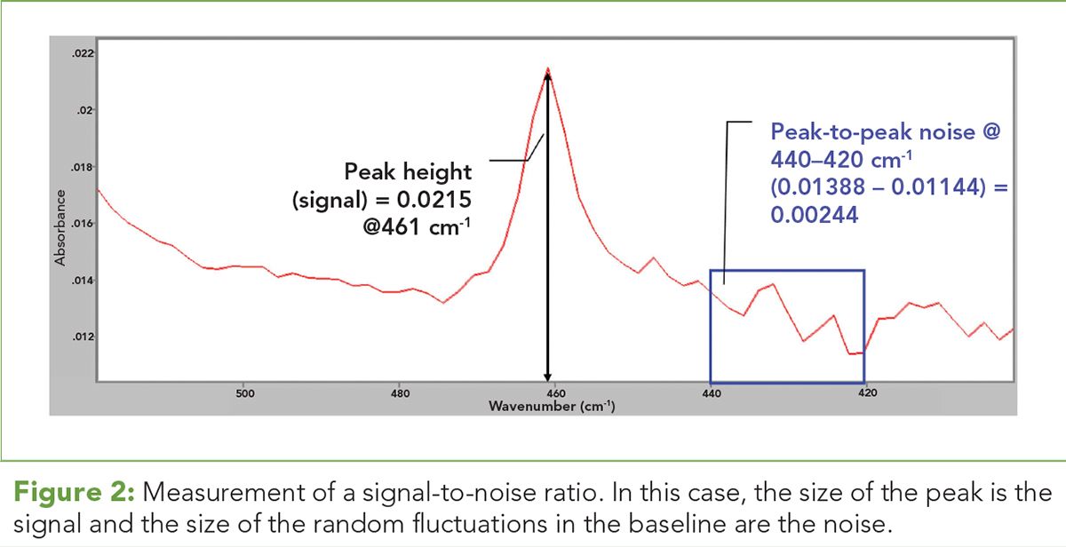
Figure 2: Measurement of a signal-to-noise ratio. In this case, the size of the peak is the signal and the size of the random fluctuations in the baseline are the noise.

A measurement of a signal-to-noise ratio, of course, needs a signal. In chromatography, spectroscopy, and other analytical techniques the signal is the magnitude of the measurement made. This is illustrated in Figure 2. (See upper right for Figure 2, click to enlarge. Figure 2: Measurement of a signal-to-noise ratio. In this case, the size of the peak is the signal and the size of the random fluctuations in the baseline are the noise.)

The y-axis in Figure 2 is in absorbance units (AU), which is a measure of the amount of light absorbed by a sample. The size of the peak at 461 cm^-1 in this case is the signal, which has a magnitude of 0.0215 AU. A measure of the error in a signal is called the peak-to-peak noise (PPN). In Figure 2, this is calculated by taking a section of the baseline and taking the highest noise point, in this case 0.01388 AU, subtracting from it the lowest noise point, which is 0.001144 AU, and obtaining a PPN of 0.00244 AU. The signal-to-noise ratio is then (0.0215) AU/(0.00244) AU for a value of ~9. This is not a particularly good SNR. Many laboratories measure what they call a limit of detection (LOD), which is typically calculated as 3x the noise in a measurement or an SNR of 3. By calculating an LOD a laboratory is saying, “this is the minimum signal I can reliably measure.” Many cannabis laboratory pesticide analysis reports, for example, contain an LOD that gives the minimum amount of a pesticide whose presence can be reliably confirmed.

However, signals at or just above the LOD are too noisy to give reliable quantitative results. So, many laboratories use a limit of quantitation (LOQ) of 10x the noise level or an SNR of 10. By calculating an LOQ a laboratory is saying, “this is the minimum amount of signal with which I can give a reliable quantitative measure.” The LOQ in a pesticide report from a cannabis analysis laboratory tells you the minimum amount of pesticide that can be reliably quantitated in a sample. Thus, the SNR of 9 in Figure 2 is above the limit of detection but below the limit of quantitation.

Random noise can be reduced by observing the same quantity multiple times and then averaging those readings. The SNR improves as the square root of the number of observations, N, averaged as such:

SNR ∝ (N)^1/2                           [2]

where N is the number of observations averaged.

In essence, equation 2 works because random noise cancels itself as N increases. Equation 2 is why we prefer to measure an average instead of a single observation, the average has the better SNR. Random error cannot be eliminated, but it can be minimized by controlling error sources and averaging data.

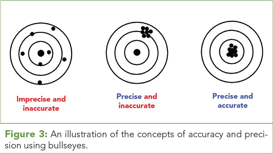
Figure 3: An illustration of the concepts of accuracy and precision using bullseyes.

Systematic Error

Systematic error occurs when a measurement is consistently wrong by the same amount and in the same direction. A classic example of systematic error is a clock that has been not been set ahead for daylight savings time. This clock will always be 1 h behind whenever you look at it. It is an example of systematic error because it is always off by the same amount, 1 h and in the same direction, always behind.

To detect systematic error, one must have a true or reference value with which to compare your observation. In the United States the reference time value is supplied by the atomic clock at the National Institute of Standards and Technology (NIST) in Gaithersburg, Maryland (3). Unlike random error, systematic error can be eliminated, in this case by simply setting the clock forward 1 h.

Accuracy and Precision

Accuracy and precision are terms in common use, and they are commonly confused. Some people seem to think they are the same thing. They are not. Precision is a measure of the scatter in a set of measurements. Accuracy is a measure of how far away a set of measurements is from the true values. This is illustrated in Figure 3. (See upper right for Figure 3, click to enlarge. Figure 3: An illustration of the concepts of accuracy and precision using bullseyes.)

Imagine you are tasked with weighing a 1.0 g standard weight on the same scale seven times. Because of error you will not get the same reading each time, but a spread of values. This is illustrated to the left in Figure 3. The bullseye represents the known value, 1.0 g, and the seven dots represent the seven readings you obtained. These readings are a random scatter and they are not particularly close to the bullseye; this data set is imprecise because the readings are widely scattered and not reproducible. This data is inaccurate because of how far on average the readings are from the bullseye, the true value. If your seven readings are about the same value, let’s say 1.9 g, they would form the plot seen in the middle of Figure 3. The readings form a tight cluster in the upper right hand corner of the bullseye, but their center is far from the true value of 1.0 in the center. This dataset is said to be precise but inaccurate. It is precise because the scatter in the data is small and the points cluster tightly together. Precision is a measure of the amount of random error in a dataset. It is found by measuring the same value on the same sample multiple times. Imprecise data will give a wide scatter, like to the left in Figure 3. Precise data will be tightly clustered as seen in the middle of Figure 3. However, this data is clustered around 1.9 g, far away from the true value of 1.0 at the center of the bullseye. Thus, this data set is inaccurate because the points fall far from the true value. Precision is a useful measure of data quality since it quantitates random error, but it ignores systematic error so it is not a complete picture. The systematic error in the middle of Figure 3 is the distance between the center of the data cluster and the bullseye.

Accuracy is a measure of the amount of random and systematic error in a data set. If the seven weights you measure all cluster tightly around 1.0 g, the diagram at the right in Figure 3 will be obtained. This data is precise because the spread of the readings is small, and it is accurate because the points cluster tightly around the true value. This is the ideal situation. Accuracy is a better measure of data quality than precision since it incorporates both random and systematic error.

Now, if one does not have a true or reference value to compare to, let’s say you lose your 1.0 g standard weight, repeated measurements on some other sample can be made to obtain a precision value. For example, you might want take a pencil and measure its weight seven times. The spread of these values will give you the precision of the balance. This is not as good as an accuracy determination, but since we do not have a standard weight, and we do not know the true weight of the pencil, the precision is the best we can do. When reporting error size in the literature, always make sure to disclose whether you are reporting an accuracy or a precision, and for an accuracy result always clearly state the source of the true value used in the calculations.

Is True Accuracy Achievable in the Cannabis Industry Right Now?

As mentioned above, obtaining an accuracy calculation requires a sample with a known value to be measured. For many industries, where plant material is processed such as tea, there exist NIST traceable standard reference materials (SRMs). For example, there exist SRMs for tea and tea extracts that can be used to give reference values for accuracy calculations (4). Since cannabis is not legal at the federal level in the United States, NIST, being a Federal agency, cannot develop cannabis SRMs for any of the materials that cannabis laboratories test. This has left the industry in the difficult position of having to develop its own standards and analytical methods.

Now, for chromatographic methods there are pure cannabinoid standards that can be used for calibration. However, since there are no SRMs available for the actual types of samples analyzed, such as cannabis buds and extracts, the effect of sample preparation on the final results is not reflected in the accuracy calculations performed. Thus, I have to conclude, perhaps controversially, that in the absence of the proper SRMs, true accuracy measurements in the cannabis analysis industry may not be possible.

This issue is reflected in the problem of inter-laboratory variation. This has been documented before and continues to be an issue (5,6). In my view, part of the problem is the lack of industry standard methods for cannabis analysis. Because of the lack of this guidance, laboratories have had to fend for themselves to develop their own methods. Thus, different laboratories have developed different ways of doing things, and this leads to different results. In particular, I have observed that many laboratories prepare samples in completely different ways, leading to variations in the results obtained.

All of this is not to say that cannabis laboratories are not precise, they are. They can get impressively reproducible data on a given sample. But until SRMs and standard methods are available, the search for a true accuracy and a solution to the inter-laboratory variation issue will, I believe, be problematic. In the meantime, it might be best for cannabis businesses to find a laboratory they trust, submit their samples to them, and only compare numbers from this chosen laboratory to themselves going forward.

References:

1. B.C. Smith, Quantitative Spectroscopy: Theory and Practice, (Elsevier, Boston, Massachusetts, 2002).
2. B.C. Smith, Fundamentals of Fourier Transform Infrared Spectroscopy, (CRC Press, Boca Raton, Florida, 2011).
3. www.time.gov.
4. www.nist.gov.
5. M.O. Bonn-Miller, M.J.E. Loflin, B.F. Thomas, J.P. Marcu, T. Hyke, and R. Vandrey, JAMA, J. Am. Med. Assoc.318, 1708 (2017).
6. B. Smith, P. Lessard, and R. Pearson, manuscript in preparation.

Brian C. Smith, PhD, is Founder, CEO, and Chief Technical Officer of Big Sur Scientific in Capitola, California. Dr. Smith has more than 40 years of experience as an industrial analytical chemist having worked for such companies as Xerox, IBM, Waters Associates, and Princeton Instruments. For 20 years he ran Spectros Associates, an analytical chemistry training and consulting firm where he taught thousands of people around the world how to improve their chemical analyses. Dr. Smith has written three books on infrared spectroscopy, and earned his PhD in physical chemistry from Dartmouth College.

How to Cite This Article

B.C. Smith, Cannabis Science and Technology1(4), 12-16 (2018).